The manufacturing processes in pharmaceutical, cosmetic, or food industries are under strict policies and regulations, and obligate manufacturers to perform constant microbiological monitoring. This means thousands of samples, usually in the form of standard Petri dishes (with microbial cultures grown on agar medium), that have to be analysed and counted manually by experienced microbiologists. This is a time-consuming and error-prone process, which requires a trained professional. To avoid these issues, an automated method applied for that task would be very appreciated.
In this article we will present deep learning methods of analysing microbiological images, developed by the NeuroSYS Research team. The crucial thing in training machine learning models is to gain large, well constructed dataset. Thus we will utilize the AGAR dataset introduced in our previous post to train a model that counts and classifies bacterial colonies grown on Petri dishes based on their RGB images.
Do you know this clue? – a dumb algorithm with lots of data beats a clever one with smaller amounts of it.
Detection of microbial colonies
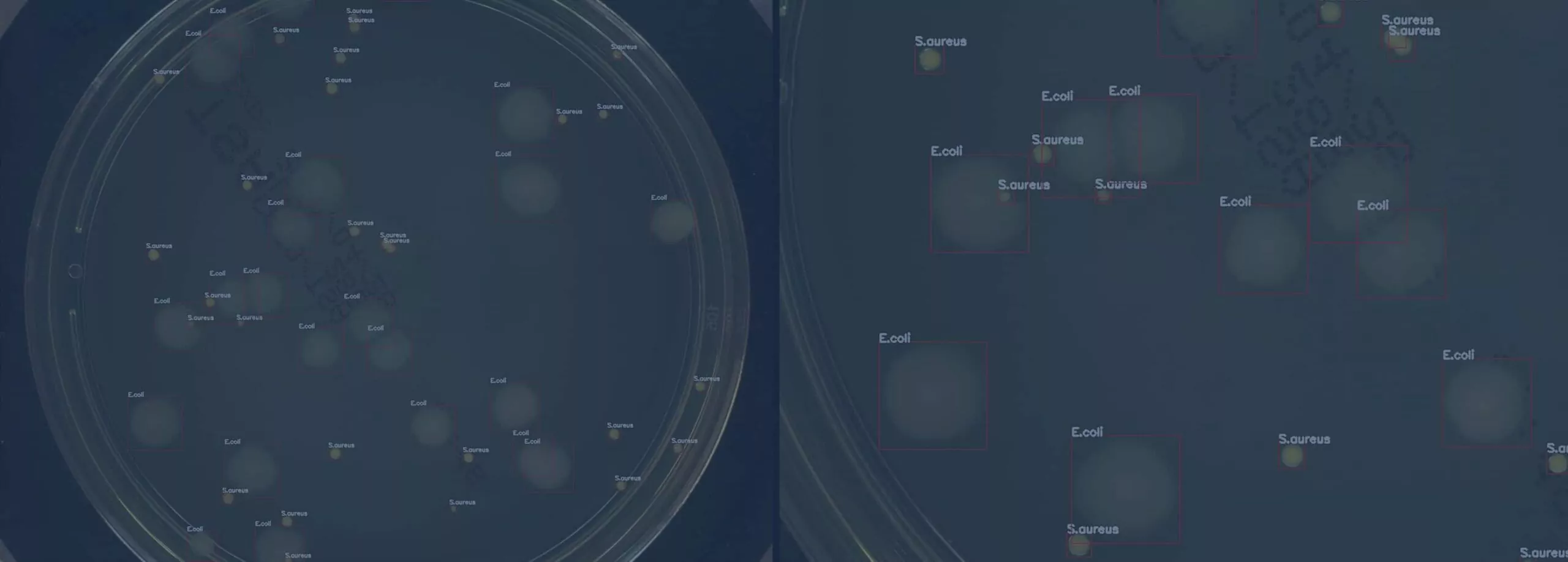
Ok, so let’s start with detecting microbes. Imagine that we have images of a Petri dish (this circle glass commonly used to keep growth medium for multiplying microbial cells in laboratories). Exemplary photos of such dishes in different setups of AGAR images are presented in the left column in Figure 1. The other 5 columns present fragments of photos (we call them patches) containing 5 different microbe types. Now it is easy to understand what microbe detection means. We simply have to determine the exact position and size of each microbe by marking it with a blue rectangle (we call it bounding box) as in Figure 1 and zoomed in Figure 2.

It seems to be easy for trained professionals, but note that microbe colony edges may be blurred, colony itself very small (even few pixel large), or camera settings (e.g. focus or lighting) very inadequate (see for example lighting conditions in 3rd row in Figure 1). Moreover some colonies may overlap which makes decisions where one colony ends and another starts very challenging. That’s why it is really difficult to build an automatic system for microbial colony localization and classification.

To do so we have developed a deep learning model for microbes detection. Deep learning is a family of AI models that utilizes mainly artificial neural networks. Such modern approaches turn out to be extremely successful in many areas, for example in computer vision or machine translation. Deep learning object detectors (in our case detecting microbial colonies) are very complicated multistage models with hundreds of layers, each consisting of hundreds of neurons.
AI tries to solve tasks that are relatively easy for humans but extremely difficult to be programmable.
Here we adopt two-stage detectors from the Region-based Convolutional Neural Network (R-CNN) family [2,3], which are known to be slow but very precise (in comparison to single-stage detectors, e.g. famous YOLO [4]). See Figure 3 for a short explanation on how it works. For a more detailed explanation of various object detection algorithms see our previous blog post on this matter.

Training the detector
After presenting the results of the microbe detection let’s check how the detector works. This contains a neural network supervised training process but not only: also data preprocessing and postprocessing is present in the training scheme in Figure 4. To train a deep learning model in a supervised manner we need a labeled dataset. As mentioned previously we use here AGAR dataset consisting of images of Petri dishes with labelled microbial colonies.
Characteristic feature of neural networks is that the model’s architecture strictly corresponds to the input size. When training (and evaluating) the network we are limited by available memory, thus we are not able to process the whole high resolution image at once, so we have to divide it into many patches. This process is not straightforward because during cutting into patches we have to ensure that a given colony appears in its entirety on at least one patch.
After that, we were prepared to train the detector (upper row in Figure 4). We selected 8 different models from the R-CNN family to make a comprehensive comparison. After the detectors were trained we tested them (lower pipeline in Figure 4) on photos (in fact on patches) unseen during the training to make sure that tests were done fairly. Note that the patches prepared for testing are simply cut off evenly—at this stage we cannot include information about where the bounding boxes lie.

Detection and counting results
We have seen in Figures 1 and 2 that our models detect colonies quite well. But how to describe the performance of detection quantitatively? There are standard numbers (metrics) that we may calculate to describe performance of the model on a test set. One of them, most popular, is called Average Precision (AP) or mean Average Precision (mAP) in case of multiclass detection (for detailed definition see this post). AP and mAP results for two selected R-CNN models (Faster ResNet-50 and Cascade HRNet) evaluated on two subsets of AGAR dataset (higher- and lower-resolution) are presented in Figure 5 (table on the left).
Generally the higher AP value the more precise detection is – the predicted and true bounding boxes better fit to each other. Note, however, that the situation is a bit complicated here because we have different microbe types which means that in addition to finding colonies, detector also needs to classify them.
Different classes of microbes are being detected with different fidelites and this affects mAP as seen in Figure 5. For example small colonies albeit with sharp edges of S. aureus bacteria are detected and marked better (AP about 65%) than big but blurred colonies of P. aeruginosa (AP about 50%) that also tend to aggregate. It is also worth mentioning that our results seem to be excellent compared to reports done with the same architectures on the famous COCO dataset: 45% for Cascade R-CNN and 37% for Faster R-CNN [5].

The final task strictly related to detection of every colony on the Petri dish is counting. After detecting all the microbial colonies we sum them up and compare this number with the ground truth number of colonies for a given Petri dish. The results for counting by the same two models on the AGAR test subsets are presented in Figure 5 (plots on the right).
On the x-axis we have the ground truth number of colonies for different dishes, estimated by trained professionals, while on the y-axis we have the value predicted by our models – each pair (truth, predicted) is represented by a single black point on these plots. It is obvious that in case of ideal predictions all points should lie on the y = x curve represented by black line. Luckily, the vast majority of points lie near this curve – the models count quite well. Two additional blue curves mark +/- 10% counting error, and we may see that only some minority of points (especially higher populated dishes with more than 50 colonies) lay outside this area.
The average counting errors were measured by the mean absolute error (MAE), defined e.g. in this blog, and so called symmetric mean absolute percentage error (sMAPE), which measures accuracy based on percentage errors [6]. In general, sMAPE do not exceed 5% which is quite a reasonable result.

Conclusions
In summary, in this article we present deep learning studies on recognition of microorganisms on Petri dishes. The selected R-CNN models perform very well in detecting microbial colonies. The detection is facilitated by the fact that the colonies have similar shapes and all species of microbes are well represented in the training data, proving the utility of the AGAR dataset. Moreover, the results obtained with base Faster R-CNN and more complex Cascade R-CNN do not differ much.
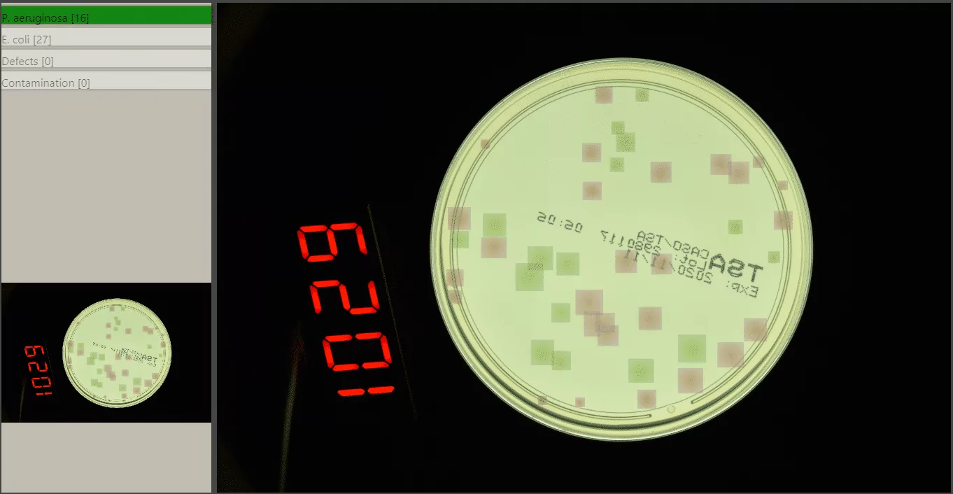
As discussed above, the detectors are more accurate for samples with less than 50 colonies. However, they still give very good estimates for dishes with hundreds or even thousands of colonies, like these presented in Figure 6, correctly identifying single colonies in highly populated samples. In the extreme case, the maximum number of detected colonies on one plate was equal to 2782. It is worth noting that it took seconds for the deep learning system, while it could take up to an hour in the case of manual counting. Moreover in some situations the detectors were able to recognize colonies difficult to see and missed by humans. These cases confirm the benefits of building an automatic microbial detection system, and that this can be successfully achieved using modern deep learning techniques.

References
[1] P. Domingos, A few useful things to know about machine learning, Commun. ACM, vol. 55, pp. 78–87, 2012.
[2] R. Girshick et al., Rich feature hierarchies for accurate object detection and semantic segmentation, Proceedings of the IEEE conference on computer vision and pattern recognition, 2014.
[3] A. Mohan, Object Detection and Classification using R-CNNs, very detailed blog on RCNN models, 2018.
[4] J. Redmon et al., You only look once: Unified, real-time object detection, Proceedings of the IEEE conference on computer vision and pattern recognition, 2016.
[5] J. Wang et al., Deep high-resolution representation learning for visual recognition, IEEE Transactions on Pattern Analysis and Machine Intelligence, 2020.
[6] S. Majchrowska, J. Pawłowski, G. Guła, T. Bonus, A. Hanas, A. Loch, A. Pawlak, J. Roszkowiak, T. Golan, and Z. Drulis-Kawa, AGAR a Microbial Colony Dataset for Deep Learning Detection, 07 July 2021, Preprint available at arXiv [arXiv:2108.01234].
Project co-financed from European Union funds under the European Regional Development Funds as part of the Smart Growth Operational Programme.
Project implemented as part of the National Centre for Research and Development: Fast Track.