The ambition behind this article
During our work in NeuroSYS, we’ve dealt with a variety of problems in Natural Language Processing, including Information Retrieval. We have mainly focused on deep learning models based on Transformers. However, Elasticsearch has often served us as a great baseline. We have been using this search engine extensively; thus, we would like to share our findings with you.
But why should you read this if you can go straight to the Elasticsearch documentation? Don’t get us wrong, the documentation is an excellent source of information, that we rely on everyday. However, as documentations do, they need to be thorough and include every bit of information on what the tool has got to offer.
Instead, we will focus more on NLP and practical aspects of Elasticsearch. We’ve also decided to split this article into two parts:
- Introductory part
- explaining main concepts,
- pointing out what we consider to be the most important,
- identifying the non-obvious things that might lead to errors or improper usage,
- Experimental part
- providing ready-to-use code,
- proposing some tips on optimization,
- presenting results of different strategies usage
Even if you are more interested in the latter, we still strongly encourage you to read the introduction.
In the following five steps, we reveal what we find to be the most important to start experimenting with your search results quality improvement.
Step 1: Understand what is Elasticsearch, and what is a search engine
Elasticsearch is a search engine, used by millions for finding query results in no time. Elastic has many applications; however, we will mainly focus on aspects most crucial for us in Natural language processing – the functionality of so-called full-text search.
Note: This article concentrates on the seventh version of Elasticsearch, as of writing this article, a more recent version 8 is already released that comes with some additional features.
Database vs. Elasticsearch
But wait, isn’t a commonly used database designed to store and search for information quickly? Do we really need Elastic or any other search engine? Well yes and no. Databases are great for fast and frequent inserts, updates, or deletes, unlike Data Warehouses or Elasticsearch.

Yes, that’s right, Elasticsearch is not a good choice when it comes to endless inserts. It’s often recommended to treat Elastic as “once built, never modified again.” It is mainly due to the way inverted indices work – they are optimized for search, not modification.
Besides, databases and Elastic differ in their use case for searching. Let’s use an example for better illustration; imagine you run a library and have plenty of books in your collection. Each book can have numerous properties associated with it, for example the title, text, author, ISBN (unique books identifier), etc., which all have to be stored somewhere, most probably in some sort of database.
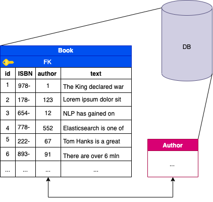
When trying to find a particular book of a given author in a query, this search is likely fast. Probably even faster if you create a database index on this field. Then it is saved on a disk in a sorted manner, which speeds up the lookup process significantly.
But what if you wanted to find all books containing a certain text fragment? In a database, we would probably look at SQL LIKE statement, possibly with some wildcards %.
Soon, further questions come along:
- What if you want to order the rows by how closely the text relates to what you queried for?
- What if you have two fields for e.g. title and text, that you would like to include in your search?
- What if you don’t want to search for the entire phrase but divide the query into separate words and accept hits containing only some of them?
- What if you want to reject the commonly occurring words in the language and consider only the relevant parts of your query?
You can probably see how problematic dealing with the more complex search is when using SQL-like queries and standard databases. That’s the exact use case for a search engine.
In short, if you want to search by ISBN, title or author, go ahead and use the database. However, if you intend to search for documents based on passages in a long text, at the same time focusing on the relevance of words, a search engine, Elasticsearch in particular, would be a better choice.
Elasticsearch manages to deal with matching queries and documents’ texts through a multitude of various query types that we’ll expand further on. However, its most important feature is an inverted index, created on terms coming from tokenized and preprocessed original texts.
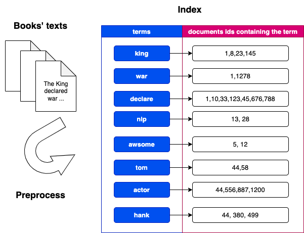
The inverted index can be thought of as a dictionary: we look for some word and get a matching description. So, here what it basically is, is a mapping from a single word/words to a whole document.
Given the previous example of a book, we would create an inverse index by taking the key words from a book’s content or the ones that describe it best, and map them as a set/vector, which from now on would represent that book.
So normally, when querying, we would have to go through each database row and check for some condition. Instead, we can break up the query into a tokenized representation (a vector of tokens) and only compare this vector to an already stored vector of tokens in our database. Thanks to that, we can also easily implement a scoring mechanism to measure how relatable all objects are to this query.
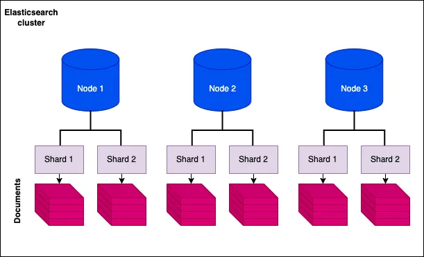
As a side note, it is also worth adding that each Elasticsearch cluster comprises many indices, which in turn contain many shards, also called Apache Lucene indices. In practice, it uses several of these shards at once to subset the data for faster querying.
Step 2: Understand when not to use Elasticsearch
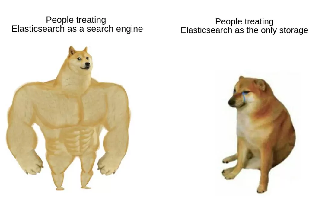
Elasticsearch is a wonderful tool; however, as in the case of many tools, when used incorrectly,, can cause as many problems as it actually solves. What we would like you to grasp from this article is that Elasticsearch is not a database but a search engine and should be treated as such. Meaning, don’t treat it as the only data storage you have. There are multiple reasons for that but we think the most important ones are:
- Search engines should only care about the data that they actually use for searches.
- When using search engines, you should avoid frequent updates and inserts.
In re 1)
Don’t pollute the search engine with stuff you don’t intend to use for searching. We know how databases grow, and schemas change with time. New data gets added causing more complex structures to form. Elasticsearch won’t be fine with it; therefore, a separate database from which you can link some additional information to your search results, might be a good idea. Besides, additional data may also influence the search results, as you will find out in the section on BM25.
In re 2)
Inverted indices are costly to create and modify. New entries in Elasticsearch enforce changes in the inverted index. The creators of Elastic have thought of that as well, and instead of rebuilding the whole index every time an update happens (eg. 10 times a second), a separate small Lucene index is created (lower level mechanism Elastic builds on). It is then merged (reindex operation) with the main one. The process takes place every second by default, but it also needs some time to complete reindexing. It takes even more time when dealing with more replicas and sharding.
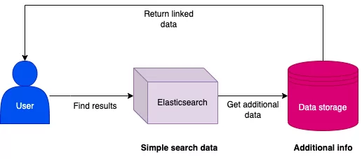
Any extra data will cause the process to take even longer. For this reason, you should only keep important search data in your indices. Besides, don’t expect the data to be immediately available, as Elastic is not ACID compliant, as it is more like a NoSQL datastore that focuses mainly on BASE properties.
Step 3: Understand the scoring mechanism
Okapi BM25
The terms stored in the index influence the scoring mechanism. BM25 is the default scoring/relevance algorithm in Elasticsearch, a successor to TF-IDF. We will not dive into the math too much here, as it would take up an entirety of the article. However, we will pick the most important parts and try to give you a basic understanding of how it works.

The equation might be a little confusing at first, but it becomes pretty intuitive when looking at each component separately.
- The first function is IDF(qi) – if you are comfortable with IDF (inverse document frequency), this one might be familiar to you. qi stands for each term from a query. What it essentially does is it penalizes the terms that are found more often in all documents by counting how many times they appear in total. We would rather take into account only the most descriptive words in a query and discard the other ones.
For example:

If we tokenized the sentence, we would expect words like Elasticsearch, search, engine, querying to be more valuable than is, a, cool, designed, for, fast, as the latter ones contribute less to the essence of this sentence.
- Another relevant factor is the function f(qi, D) or frequency of the term qi within document D, for which the score is being counted. Intuitively, the higher the frequency of query terms within a particular document, the more relevant this document is.
- Last but not least is fieldLen/avgFieldLen ratio. It calculates how long a given document is compared with the average length of all documents stored. Since it is placed in a denominator we can observe that the score will decrease with the document’s length growth, and vice versa. So if you are experiencing more short results than longer ones it is simply because this factor boosts shorter texts.

Step 4: Understand the mechanism of text pre-processing
Analyzers
Probably the first question you’d need to raise when thinking of optimization is: how the texts are preprocessed and represented within your inverted index. There are many ready-to-use concepts in Elasticsearch, which are taken from Natural Language Processing. They are encapsulated within so-called analyzers that change the continuous text into separate terms, which are indexed instead. In “Layman’s terms”, an analyzer is both a Tokenizer, which divides the text into tokens (terms), and a collection of Filters, which do additional processing.
We can use built-in Analyzers provided by Elastic, or define our own. In order to create a custom one, we should determine which tokenizer we’d like to use and provide a set of filters.
We can apply three possible analyzers’ types to a given field, which varies based on how and when they process text:
- indexing analyzer – used during the document indexing phase,
- search analyzer – used to map query terms during the search, so they can be compared to terms indexed in a field. Note: if we don’t explicitly define the search analyzer, by default, the indexing analyzer for this field will be used instead
- search quote analyzer – used for strict search of full phrases
Usually, there is no point in applying a search analyzer different from an indexing analyzer. Additionally, if you would like to test them yourself, it can be easily done via the built-in API or directly from the library in the language of your choice.
The built-in analyzers should be able to cover the most often used operations applied during indexing. If needed, you can use analyzers that are explicitly made for a specific language, called Language analyzers.
Filters
Despite their name, Filters not only perform token selection but are also responsible for a multitude of common NLP preprocessing tasks. They can also be used for a number of operations such as:
- stemming,
- stopwords filtering,
- lower/upper casing,
- n-grams creation on chars or words.
However, they cannot perform lemmatization. Below, we’ve listed some of the most common ones. However, if you’re interested in the complete list of available filters, you can find it here.
- shingle – creates n-grams of words,
- n-gram – creates n-grams of characters,
- stop-words – removes stopwords,
- stemmer (Porter/Lovins) – performs stemming according to the Porter/Lovins algorithm,
- remove_duplicate – removes duplicate tokens.
Tokenizers
They aim to divide the text into tokens according to a selected strategy, for example:
- standard_tokenizer – removes punctuation and breaks text based on words boundaries,
- letter_tokenizer – breaks text on each non-letter character,
- whitespace_tokenizer – breaks text on any whitespace,
- pattern_tokenizer – breaks texts on specified delimiter e.g., semicolon or comma.
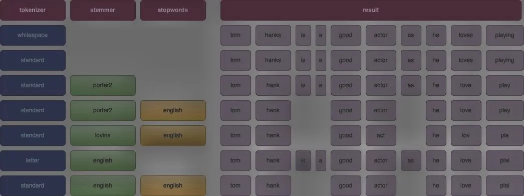
In the diagram below, we present some exemplary analyzers and their results on the sentence “Tom Hanks is a good actor, as he loves playing.”
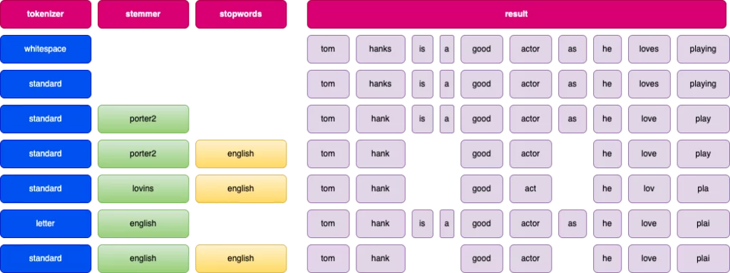
Each tokenizer operates differently, so pick the one that works best for your data. However, a standard analyzer is usually a good fit for many scenarios.
Step 5: Understand different types of queries
Queries
Elasticsearch enables a variety of different query types. The basic distinction we can make is whether we care about the relevance score or not. Having this considered, we have got two contexts to choose from:
- query context – calculates the score, whether the document matches a query, and how good is the match,
- filter context – does not calculate the score, it only identifies the documents that match the query or not.
So, use a query context to tell how closely documents match the query and a filter context to filter out unmatched documents that will not be considered when calculating the score.
Bool query
Even though we’ve already stated that we will mainly focus on text queries, it’s essential to at least understand the basics of Bool queries since match queries boil down to them. The most significant aspect is the operator we decide to use. When creating queries, we would often like to use logical expressions like AND, OR, NOR. They are available in Elasticsearch DSL (domain specific language) as must, should, and must_not, respectively. Using them we can easily describe the required logical relationships.
Full text queries
These are the ones we are most interested in, since they are ideal for fields containing text on which an analyzer has been applied. It is worth noting that when querying each field during a search, the query text will also be processed with the same analyzer used for indexing the field.
There are several types of FTS queries:
- intervals – Uses rules for matching terms, and allows for their ordering. What the query excels in is proximity searches. We are able to define an interval (since the query name) where we can look for some terms. Useful, especially when we know that the searched terms will not necessarily occur together but might appear in a predefined distance from each other. Or on the contrary, we want them to stay close together.
- combined_fields – This type allows for querying multiple fields and treating them as if they were combined. For example: when querying for the first name and the last name which we might want to be paired.
- query_string – A lower level query syntax. It allows for creating complex queries using operators like AND, OR, NOT, as well as, multiple fields querying or multiple additions like wildcard operators.
- simple_query_string – It’s a higher level wrapper for a query_string, which is more end-user friendly.
- match – “the go-to” choice for FTS, the subtypes are:
- match_phrase – designed for “exact phrases” and word proximity matching,
- multi_match – a match type that allows for querying multiple fields in a preffered manner.
We will now focus on explaining Match based queries in more detail, as we find them versatile enough to do everything we need while being pretty quick to write and modify.
Match query – this is a standard for full-text searches, where each query is analyzed the same way as the field it is matched against. We find the following parameters to be the most important ones:
- Fuzziness – when searching for some phrases users can make typos. Fuzziness enables to deal quickly with such spelling errors searching for similar words at the same time. It defines the accepted error rate for each word, which is interpreted as Levenstein edit distance. Fuzziness is an optional parameter and can take values such as 0, 1, 2, or AUTO. We recommend keeping the parameter as AUTO since it automatically adjusts how many errors can be made per word depending on its length. The error distance is 0, 1, and 2 for 2, 3-5, and over 5 characters word length, respectively. If you decide to use synonyms in a field, fuzziness cannot be used anymore.
- Operator – as mentioned above, a boolean query is constructed based on the analyzed search text. This parameter defines which operator AND or OR will be used, and defaults to OR. For example, the text “Super Bitcoin mining” for OR operator is constructed as “Super OR Bitcoin OR mining,” while for AND, it is built as “Super AND Bitcoin AND mining.”
- Minimum_should_match – this defines how many of the terms in a boolean query should be matched for the document to be accepted. It is quite versatile as it accepts integers, percentages, or even their combinations.
Match phrase query – it’s a variation of match query where all terms must appear in the queried field, in the same order, next to each other. The sequence can be modified a bit when using an analyzer that removes stopwords.
Match prefix query – it converts the last term in the query into a prefix term, which acts as a term followed by a wildcard. There are two types of this query:
- Match boolean prefix – from the terms a boolean query is constructed,
- Match phrase prefix – the terms are treated as a phrase; they need to be in specific order.
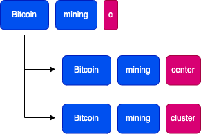
When using a match phrase prefix query, “Bitcoin mining c” would be matched with both documents “Bitcoin mining center”, as well as “Bitcoin mining cluster”, since the first two words form a phrase, while the last one is considered as a prefix.
Combined fields query – allows for searching through multiple fields as if they were combined into a single one. Clarity is a huge advantage of combined fields query, since when creating this type of a query it is converted to a boolean query and chosen logical operators are used. However, there is one important assumption for combined fields query; all queried fields require the same analyzer.
The disadvantage of this query is the increased search time, as it must combine fields on the fly. That’s why, it might be wiser to use copy_to when indexing documents.
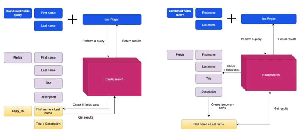
Copy_to allows for creating separate fields which combine data from other fields. Which translates into no additional overhead during searches.
Multi match query – it differs from combined fields, since it enables querying multiple fields that have different analyzers applied or even of a different type. The most important parameter is the type of a query:
- best_fields – a default value, it calculates the score in each of the specified fields. Useful when we want the answer to appear in only one of the given fields instead of the terms to be found in multiple fields.
- most_fields – the best when the same text can be found in different fields. Different analyzers might be used on those fields, one of them can have stemming and synonyms, while the second can use n-grams, and the last one, the original text. The relevance score combines all fields’ scores and then is divided by the number of matches in each field.
Note: best_fields and most_fields are treated as FIELD centric, meaning that matches in a query are applied per field instead of per term. For example, query “Search Engine” with operator AND means that all terms must be present in a single field, which might not be our intention.
- cross_fields – is considered to be TERM centric and is a good choice when we expect the answer to be found in multiple fields. Such as, when querying for the first and the last name, we would expect to find them in different fields. Compared to most and best fields, where the terms MUST be found in the same field, here, all terms MUST be placed in at least one field. One more cool thing about cross_fields is that it can group together the fields with the same analyzer, and calculate scores on groups instead. More details can be found in the official documentation.
Boosting
We would also like to highlight that queries can be boosted. We use this feature extensively on a daily basis.

This query would multiply the score for the field Title by 2 times, Author by 4 times while Description score will remain unboosted. Boost can be an integer or a floating point number; however it must be greater or equal to 1.0.
Conclusion
To sum up, we’ve presented five steps we find crucial to start working with Elastic. We’ve discussed what Elasticsearch is, and what it isn’t, and how you’re supposed to and not supposed to use it. We’ve also described the scoring mechanism and various types of queries and analyzers.
We are confident that the knowledge collected in this article is essential to start optimizing your search results. The article was intended as an introduction to some key concepts, but also as a foundation for the next one, in which we will provide you with examples of what is worth experimenting with, and will share the code.
We hope that this blog post gave you some insight on how different search mechanisms work. We hope you’ve learned something new or handy, which one day you might find useful in your projects.
